@Jeffrey Curl, your original post here was an excellent one in that it explained what you were doing in detail. I wanted to respond to you on first read but I dod't have the time to do a proper job of it. When I came back to it
@RegionRat had posted and covered what I had planned on commenting on.
I want to expand on a couple of things that are important to understand and will hopefully help you down the road. The first has to do with the Satterlee Test or Ladder. To understand the fallacy of the test you have to understand the nature of statistics from both a testing and probability standpoint. Suffice it to say that when choosing samples from a large lot of ammunition (or loading individual rounds) you are using different components each shot so all of the factors that affect velocity are different and independent in how their different effects combine. This leads to different combinations of effects and this shows up in variations in velocity and is measured by standard deviation of the mean velocity when multiple values are measured and averaged. Let's assume you had a load that you shot a large number ( population) of shots over a chronograph over time that had an average mean velocity of 2730 fps and a standard deviation of 7 fps. If you were to load 100 rounds (sample) using the exact same procedures one example of the data would look like this. Loading just one round is no different than picking one from the 100.

In this case there are 54 shots greater than the true mean of sample and 46 less than the true mean of the samples. When you pick or load any one round you don't know which one you will get. The end result if you load one round of a charge and another round of another charge it is entirely possible to get one high and the other low so that the velocity between the 2 can be exaggerated as being higher or lower than what addition data would show. In this case the extreme speed is 41 fps.
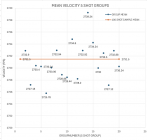
This is why the Satterlee method is flawed and also why as the chart weight increment decreases the likkehood of flat spots increases.
So what happens if we load more and average the velocities for each load? Typically the thought is 3 or five shot groups. The following shows one possible combinations 5 shot averages of the above data.
The five shot groups are closer to average of the 100 shots but still have a spread of almost 15 fps. In this example of one hundred shots these are 20 of the possible approximately 75,000,000 possible random combinations!
If those 100 shots were analyzes as 20 shot groups one possible result is

Notice that each of the groups is much closer to the true sample mean. Again this is only five of the possible results of 20 shot groups out of the possible 535,983,370,403,809,682,970 possible combinations. Notice that the spread is now only about 4 fps.
And so it goes. This is a demonstration of how sample size is important in trying to interpret and analyze specific test data. In and of itself it is not about statistically significant data. That term comes into play when comparing test data between tests and to known standards.
Now that we have data (the test data is velocity) we need to look at how the individual data points vary from the mean. This is measured by the Variance or Standard Deviation of the Mean. In the above example of the 5 shot group the Standard Deviation is shown below

and for the 20 shot group below

The above examples demonstrate some universal observations about sample size. In the case of mean or average the number of data sample points has an affect on the how accurate the prediction of velocity of the large group can be and how accurate the sample mean represents the much larger population. It also demonstrates that the larger the sample size the greater the extreme spread is likely to be because you increase the likelihood of finding an extreme value.
The second and more important observation is how small sample sizes bias the standard deviations on the low side of the true value and also how more sample points decrease the spread of the sample data variation from the larger sample size and the true population standard deviation.
This example is based on velocity data but it would also apply to group size and mean radius or any other direct measurement of a variable.